< Previous lesson | Overview | Next lesson >
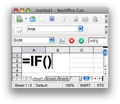
=IF()
How to set conditions for your formulas
=IF() is a formula used for performing something under certain conditions. It might seem like it is quite similar to =SUMIF(), but =IF() is a lot more versatile. In short, you make a statement (any statement that can be either TRUE or FALSE), and have Calc perform one task if it is TRUE, and another task if it is FALSE.
The syntax for =IF() is as follows:
=IF([Any statement that can be either TRUE or FALSE];[If the statement is TRUE, perform this]; [If the statement is FALSE, perform this])
As you can see, this formula has three parameters, where the first one is a test, and the next two defines what to do if the first parameter is either true or false.
We start off with some theory, as usual, before we start typing.
Now take a closer look at the first parameter:
[Any statement that can be either TRUE or FALSE]
This test can be a variety of statements, as long as it can be either TRUE or FALSE. This means that all of these are valid:
- 2+2=4
- A1=12
- SUM(A1:C42)
- A2=A5*12
- TRUE
- FALSE
This time look at the second parameter:
[If the statement is TRUE, perform this]
If the first parameter is TRUE, this parameter will tell Calc what to do next. You can put a value or formula here, such as:
- 53*12
- A$4+$A$12
- B5*12
- SUM(A1:A1000)
- AVERAGE(C50:C100)
- VLOOKUP(A1;B1:D100;3;0)
As you might see, this opens up for a lot of exciting possibilities! This is one of the real strengths of a spreadsheet; it is relatively easy to ad some level of intelligence.
Do you see something peculiar about the formulas above? None of them start with an "=". This is intentional, as you do not need to start a formula with "=" as long as it is used inside another formula.
Now look at the third an final parameter:
[If the statement is FALSE, perform this]
If the first parameter is FALSE, this parameter will tell Calc what to do next. You can put a value or formula here, such as:
- 53*12
- A$4+$A$12
- B5*12
- SUM(A1:A1000)
- AVERAGE(C50:C100)
- VLOOKUP(A1;B1:D100;3;0)
As you see, this is very much the same as with the previous parameter.
But let us ad something here; it is very common to ad yet another IF()-statement in the final parameter. It can also be used in the second parameter, but most feel it gives a better structure to ad it to the final parameter. We will go further into this in a later lesson.
Finally, we are done with the theory, now we can start using it...
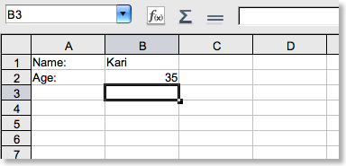
In A1, type "Name:", in B1 type "Kari", in A2, type "Age:" and in B2 type "35", as shown above.
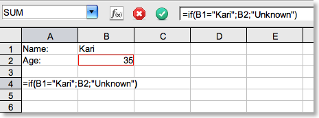
In cell A4, enter the formula as shown above.
Then hit [Enter]. If everything is typed correctly, it should show 35.
First Calc checks wether [B1="Kari"] is correct. If it is, it will show the contents of [B2]. Otherwise, it will show the word Unknown, hence ["Unknown"].
When working with text, it is very important to use the " at the beginning and end of the text string inside formulas.
Change the name in B1 to "Steven", hit [Return] and observe what happens.
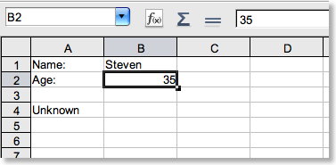
The value in A4 changed to "Unknown", which is what the third parameter states.
Now I really encourage you to experiment with this formula, as this will help you leverage some of the phenomenal powers of Calc! Try putting a cell-reference or another formula in the first parameter, try entering a number-value in the second parameter etc.